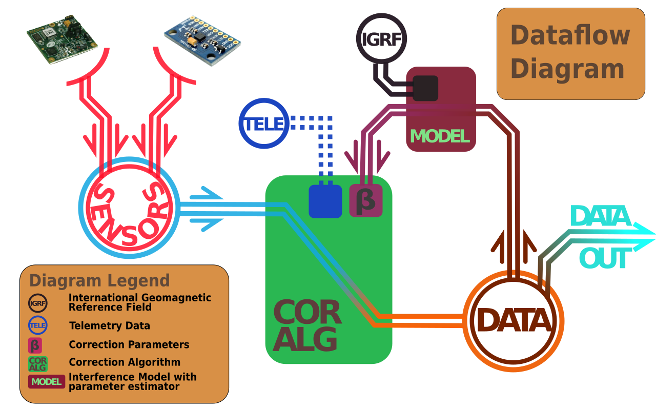
On the input from my mentor, I dedicated a bit of time and made a dataflow diagram for the correction algorithm I intend to implement in the coming weeks. It makes the overall design and flow of information much clearer to anyone not in the mood to read on all specifics of the algorithm.

As I’ve mentioned in the BeagleSat video, which you should definitely check out, the purpose of the algorithm is to reduce interference from local magnetic sources, isolating the sensor measurements from the spacecraft. In effect, eliminating the need to pack long (and heavy) sensor booms on a CubeSat, which is both convenient design wise and reduces expenses.

So how does this thing work?

Here’s a brakedown of what you can see on the image above:

• Each sensor is polled for raw sensor readouts which are stored in the database (DATA)
• Once a calibration is requested and a representative body of data is available, it gets sent to the parameter estimator (MODEL)
• The estimator fits the data to a model based on the IGRF and computes the correction parameters (Beta)
• The correction parameters are stored in the correction algorithm (Corr. Alg) to compensate for time-invariant errors in the incoming sensory data
• Telemetry data can be used in addition to the correction parameters to enable compensation for larger time-variant sources of on-board interference

The correction algorithm is doing linear operations on the incoming data to provide compensated readouts to the database, which get stored alongside the raw data. The raw data is used if a re-calibration is required to get new correction parameters.

The really interesting part goes on in the parameter estimator.

It works on the premise that if one was to plot the output of an ideal or error free three-axis sensor that was rotated freely through various orientations, those plot points would fall on the surface of a sphere. In case where these points do not fall on a sphere but on a distorted ellipsoid, that signifies that there are imperfections in the sensor or magnetic fields that interfere with the measurements. In a simpler 2D example, the sensor readouts would, in the ideal case, fall on a circle, or in the case of the sensor with interference a distorted ellipse.

The model is derived from the IGRF as a sphere with a radius equal to the magnitude of the estimated Earth’s magnetic field at that point. The raw data, which should have a representative body of readouts containing samples from various orientations of the sensor, is then fitted to this sphere using a batch least-square computation to estimate the correction parameters required to compensate for the errors in the readouts.

The correction parameters are able to successfully compensate for all static sources of magnetic interference. To be able to correct for time varying magnetic sources on-board the spacecraft, such as solar panels or communication equipment, the correction algorithm is further strengthened by including correction factors based on the telemetry data from the spacecraft.

For an in-depth review of the algorithms used (and cool graphs), refer to these publications:

• Clavier, Odile, Theodore Beach, Brynmor Davis, Ariane Chepko, James Cutler, “Enabling low-cost, high accuracy magnetic field measurements on Small Sats for space weather missions”, 25th Small Satellite Conference, Logan, Utah, August, 2011.

• Elkaim, G. and C. Foster, “Extension of a Nonlinear, Two-Step Calibration Methodology to Include Non Orthogonal Sensor Axes,” IEEE Transactions on Aerospace Electronic Systems, Vol. 44, No. 3, July 2008.

• Gebre-Egziabher, D., G. H. Elkaim, J. D. Powell and B.W. Parkinson, “Calibration of Strapdown Magnetometers in the Magnetic Field Domain,” Journal of Aerospace Engineering, Vol. 19, No. 2, pp. 6–16, 2006.