I’ve been working on test code for the sensor data correction algorithm that I mentioned a while ago and I’ve cracked it last night. (woohoo!)

The original research was quite easy to follow, although a bit of verbosity on the equations side wouldn’t have hurt.

How good is the correction algorithm? Well, judge for yourself.

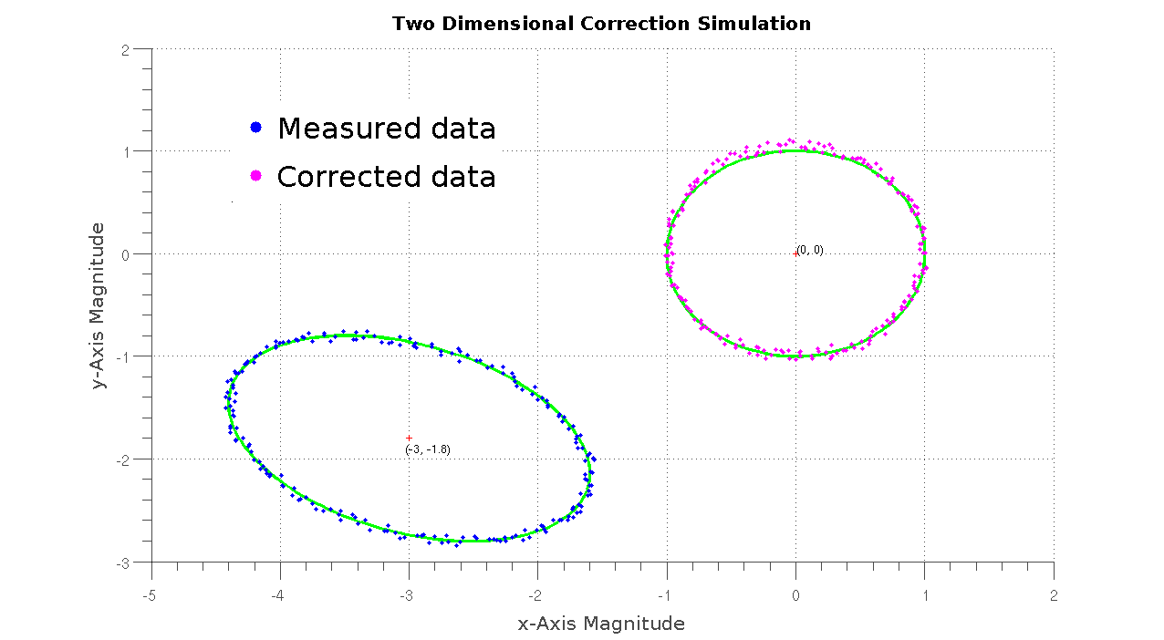
The “measured” data, seen here in blue, was simulated by adding a bunch of distortion elements to an otherwise normal set of ellipse points, eg. rotation, scaled axes and displaced center. The data was fuzzed further by adding 5% noise to the data points.

The measured data is then fitted to a distorted ellipse using a batch linear least-square algorithm to extract the correction factors needed to compensate for the errors introduced in the measured data. Once computed, the correction factors are used on the data set to obtain the corrected data set, seen here in magenta. The image is fitted with two green ellipses, one distorted and one optimal for comparison with the two presented data sets.

All in all, the algorithm works as expected and gives astoundingly good estimates for the correction factors. The rotation angle parameter is the only outlier, with an error range below 0.2 rads, the other factors usually range well below 1%.

Next up, expanding the algorithm to 3-axis data and adding time-varying error correction in the mix.